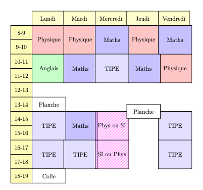
画弧线
\begin{tikzpicture}[xscale=6,yscale=6]
\draw[<->] (0,0.8) -- (0,0) -- (0.8,0);
\draw[green,thick,domain=0:0.5]
plot(\x, {0.025+\x*\x});
\draw[red, thick, domain=0:0.5]
plot(\x, {sqrt(\x)});
\draw[blue, thick, domain=0:0.5]
plot(\x, {abs(\x)});
\end{tikzpicture}
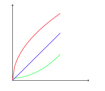
画球体
\begin{tikzpicture}
\draw[step=1,color=gray!40] (-2,-2) grid (2,2);
\draw[->] (-3,0) -- (3,0);
\draw[->] (0,-3) -- (0,3);
\draw[color=gray!40] (0,0) circle (1); %
\draw[color=red] (1,0) arc (0:45:1);
\draw[color=gray!40] (0,0) ellipse (1 and 0.5);
\draw[color=green] (1,0) arc (0:60:1 and 0.5);
\end{tikzpicture}
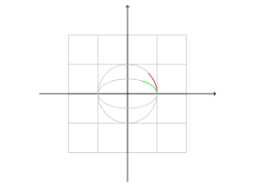
流程图
\usetikzlibrary{positioning, shapes.geometric}
\begin{tikzpicture}[node distance=10pt]
  \node[draw, rounded corners]                        (start)   {Start};
  \node[draw, below=of start]                         (step 1)  {Step 1};
  \node[draw, below=of step 1]                        (step 2)  {Step 2};
  \node[draw, diamond, aspect=2, below=of step 2]     (choice)  {Choice};
  \node[draw, right=30pt of choice]                   (step x)  {Step X};
  \node[draw, rounded corners, below=20pt of choice]  (end)     {End};

  \draw[->] (start)  -- (step 1);
  \draw[->] (step 1) -- (step 2);
  \draw[->] (step 2) -- (choice);
  \draw[->] (choice) -- node[left]  {Yes} (end);
  \draw[->] (choice) -- node[above] {No}  (step x);
  \draw[->] (step x) -- (step x|-step 2) -> (step 2);
\end{tikzpicture}
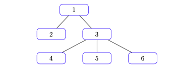
树
\begin{tikzpicture}[sibling distance =80pt]
  \tikzset{
    box/.style ={
      rectangle, %矩形节点
      rounded corners =5pt, %圆角
      minimum width =50pt, %最小宽度
      minimum height =20pt, %最小高度
      inner sep=5pt, %文字和边框的距离
      draw=blue %边框颜色
    }}

  \node[box] {1}
  child {node[box] {2}}
  child {node[box] {3}
    child {node[box] {4}}
    child {node[box] {5}}
    child {node[box] {6}}
  };
\end{tikzpicture}
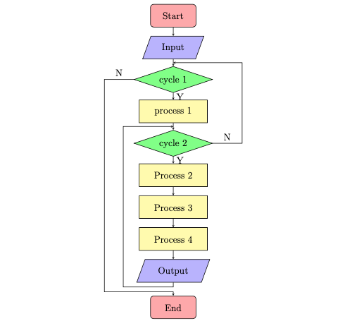
流程图4
\usetikzlibrary{positioning, shapes.geometric}
\usetikzlibrary{calc}

% Define the basic shape of flow chart
\tikzstyle{startstop} = [rectangle, rounded corners, minimum width = 2cm, minimum height=1cm,text centered, draw = black, fill = red!30]
\tikzstyle{io} = [trapezium, trapezium left angle=70, trapezium right angle=110, minimum width=2cm, minimum height=1cm, text centered, draw=black, fill = blue!25]
\tikzstyle{process} = [rectangle, minimum width=3cm, minimum height=1cm, text centered, draw=black, fill = yellow!35]
\tikzstyle{decision} = [diamond, aspect = 3, text centered, minimum width = 2.5cm, draw=black, fill = green!45]
% arrow shape
\tikzstyle{arrow} = [->,>=stealth]

\setlength{\PreviewBorder}{0.5bp}

\centering
\begin{tikzpicture}[node distance = 1.2cm]
  % Define flowchart  shape
  \node (start) [startstop] {Start};
  \node (in1) [io, below of = start, yshift=-0.2cm, minimum width=1cm] {Input};
  \node (dec1) [decision, below of=in1, yshift=-0.2cm] {cycle 1};
  \node (pro1) [process, below of=dec1,yshift=-0.2cm] {process 1};
  \node (dec2) [decision, below of=pro1, yshift=-0.2cm] {cycle 2};
  \node (pro2) [process, below of=dec2,yshift=-0.2cm] {Process 2};
  \node (pro3) [process, below of=pro2,yshift=-0.2cm] {Process 3};
  \node (pro4) [process, below of=pro3,yshift=-0.2cm] {Process 4};
  \node (in2)  [io, below of=pro4, yshift=-0.2cm] {Output};
  \node (stop) [startstop, below of=in2,node distance = 1.6cm] {End};
  % connect
  \draw[arrow] (start)  -- (in1);
  \draw[arrow] (in1) -- (dec1);
  \draw[arrow] (dec1.west)-- node[anchor=south] {N} ($(dec1.west) - (1.3,0)$) |- ($(stop.north)!.3!(in2.south)$) -- (stop);
  \draw[arrow] (dec1) -- node[anchor=west] {Y} (pro1);
  \draw[arrow] (pro1) -- (dec2);
  \draw[arrow] (dec2.east) -- node[anchor=south] {N} ($(dec2.east) + (1.3,0)$) |- ($(in1.south)!.5!(dec1.north)$);
  \draw[arrow] (dec2) -- node[anchor=west] {Y} (pro2);
  \draw[arrow] (pro2) -- (pro3);
  \draw[arrow] (pro3) -- (pro4);
  \draw[arrow] (pro4) -- (in2);
  \draw[arrow] (in2.south)  -- ($(in2.south)-(0,0.2)$) -- ($(in2.south) - (2.2,0.2)$) |- ($(pro1.south)!.5!(dec2.north)$);
\end{tikzpicture}
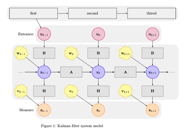
使用matrix和path画结构接近矩形的图
% Kalman filter system model
% by Burkart Lingner
% An example using TikZ/PGF 2.00
%
% Features: Decorations, Fit, Layers, Matrices, Styles
% Tags: Block diagrams, Diagrams
% Technical area: Electrical engineering

\documentclass[a4paper,10pt]{article}

\usepackage[english]{babel}
\usepackage[T1]{fontenc}
\usepackage[ansinew]{inputenc}

\usepackage{lmodern}	% font definition
\usepackage{amsmath}	% math fonts
\usepackage{amsthm}
\usepackage{amsfonts}

\usepackage{tikz}
\usetikzlibrary{decorations.pathmorphing} % noisy shapes
\usetikzlibrary{fit}					% fitting shapes to coordinates
\usetikzlibrary{backgrounds}	% drawing the background after the foreground
\usetikzlibrary[positioning]
\begin{document}

\begin{figure}[htbp]
\centering
% The state vector is represented by a blue circle.
% "minimum size" makes sure all circles have the same size
% independently of their contents.

\tikzstyle{state}=[circle,
                                    thick,
                                    minimum size=1.2cm,
                                    draw=blue!80,
                                    fill=blue!20]

% The measurement vector is represented by an orange circle.
\tikzstyle{measurement}=[circle,
                                                thick,
                                                minimum size=1.2cm,
                                                draw=orange!80,
                                                fill=orange!25]

% The control input vector is represented by a purple circle.
\tikzstyle{input}=[circle,
                                    thick,
                                    minimum size=1.2cm,
                                    draw=purple!80,
                                    fill=purple!20]

% The input, state transition, and measurement matrices
% are represented by gray squares.
% They have a smaller minimal size for aesthetic reasons.
\tikzstyle{matrx}=[rectangle,
                                    thick,
                                    minimum height=1cm,
                                    minimum width=2cm,
                                    draw=gray!80,
                                    fill=gray!20]

% The system and measurement noise are represented by yellow
% circles with a "noisy" uneven circumference.
% This requires the TikZ library "decorations.pathmorphing".
\tikzstyle{noise}=[circle,
                                    thick,
                                    minimum size=1.2cm,
                                    draw=yellow!85!black,
                                    fill=yellow!40,
                                    decorate,
                                    decoration={random steps,
                                                            segment length=2pt,
                                                            amplitude=2pt}]

% Everything is drawn on underlying gray rectangles with
% rounded corners.
\tikzstyle{background}=[rectangle,
                                                fill=gray!10,
                                                inner sep=0.2cm,
                                                rounded corners=5mm]

\begin{tikzpicture}[>=latex,text height=1.5ex,text depth=0.25ex]
    % "text height" and "text depth" are required to vertically
  % align the labels with and without indices.
  \tikzstyle{myrec}=[rectangle,draw, minimum height=1cm,minimum width=4.5cm, anchor=north west,text centered]
  % The various elements are conveniently placed using a matrix:
  \matrix[row sep=0.5cm,column sep=0.5cm] {
    % First line: Control input
    &
        \node (u_k-1) [input]{$\mathbf{u}_{k-1}$}; &
        &
        \node (u_k)   [input]{$\mathbf{u}_k$};     &
        &
        \node (u_k+1) [input]{$\mathbf{u}_{k+1}$}; &
        \\
        % Second line: System noise & input matrix
        \node (w_k-1) [noise] {$\mathbf{w}_{k-1}$}; &
        \node (B_k-1) [matrx] {$\mathbf{B}$};       &
        \node (w_k)   [noise] {$\mathbf{w}_k$};     &
        \node (B_k)   [matrx] {$\mathbf{B}$};       &
        \node (w_k+1) [noise] {$\mathbf{w}_{k+1}$}; &
        \node (B_k+1) [matrx] {$\mathbf{B}$};       &
        \\
        % Third line: State & state transition matrix
        \node (A_k-2)         {$\cdots$};           &
        \node (x_k-1) [state] {$\mathbf{x}_{k-1}$}; &
        \node (A_k-1) [matrx] {$\mathbf{A}$};       &
        \node (x_k)   [state] {$\mathbf{x}_k$};     &
        \node (A_k)   [matrx] {$\mathbf{A}$};       &
        \node (x_k+1) [state] {$\mathbf{x}_{k+1}$}; &
        \node (A_k+1)         {$\cdots$};           \\
        % Fourth line: Measurement noise & measurement matrix
        \node (v_k-1) [noise] {$\mathbf{v}_{k-1}$}; &
        \node (H_k-1) [matrx] {$\mathbf{H}$};       &
        \node (v_k)   [noise] {$\mathbf{v}_k$};     &
        \node (H_k)   [matrx] {$\mathbf{H}$};       &
        \node (v_k+1) [noise] {$\mathbf{v}_{k+1}$}; &
        \node (H_k+1) [matrx] {$\mathbf{H}$};       &
        \\
        % Fifth line: Measurement
        &
        \node (z_k-1) [measurement] {$\mathbf{z}_{k-1}$}; &
        &
        \node (z_k)   [measurement] {$\mathbf{z}_k$};     &
        &
        \node (z_k+1) [measurement] {$\mathbf{z}_{k+1}$}; &
        \\
    };
  \node[myrec] (myr) at (-8, 6) {first};
  \node[myrec] (myr2) [right = of myr] {second};
  \node[myrec] (myr3) [right = of myr2] {third};

    % The diagram elements are now connected through arrows:
    \path[->]
        (A_k-2) edge[thick] (x_k-1)	% The main path between the
        (x_k-1) edge[thick] (A_k-1)	% states via the state
        (A_k-1) edge[thick] (x_k)		% transition matrices is
        (x_k)   edge[thick] (A_k)		% accentuated.
        (A_k)   edge[thick] (x_k+1)	% x -> A -> x -> A -> ...
        (x_k+1) edge[thick] (A_k+1)

        (x_k-1) edge (H_k-1)				% Output path x -> H -> z
        (H_k-1) edge (z_k-1)
        (x_k)   edge (H_k)
        (H_k)   edge (z_k)
        (x_k+1) edge (H_k+1)
        (H_k+1) edge (z_k+1)

        (v_k-1) edge (z_k-1)				% Output noise v -> z
        (v_k)   edge (z_k)
        (v_k+1) edge (z_k+1)

        (w_k-1) edge (x_k-1)				% System noise w -> x
        (w_k)   edge (x_k)
        (w_k+1) edge (x_k+1)

        (u_k-1) edge (B_k-1)				% Input path u -> B -> x
        (B_k-1) edge (x_k-1)
        (u_k)   edge (B_k)
        (B_k)   edge (x_k)
        (u_k+1) edge (B_k+1)
    (B_k+1) edge (x_k+1)
    (myr) edge (myr2)
    (myr2) edge (myr3)
    (myr) edge (u_k-1)
        ;

    % Now that the diagram has been drawn, background rectangles
    % can be fitted to its elements. This requires the TikZ
    % libraries "fit" and "background".
    % Control input and measurement are labeled. These labels have
    % not been translated to English as "Measurement" instead of
    % "Messung" would not look good due to it being too long a word.
    \begin{pgfonlayer}{background}
        \node [background,
                    fit=(u_k-1) (u_k+1),
                    label=left:Entrance:] {};
        \node [background,
                    fit=(w_k-1) (v_k-1) (A_k+1)] {};
        \node [background,
                    fit=(z_k-1) (z_k+1),
                    label=left:Measure:] {};
         \node [background,
                    fit=(myr) (myr3)] {};
    \end{pgfonlayer}
\end{tikzpicture}

\caption{Kalman filter system model}
\end{figure}

\end{document}
这个图中,用到了矩阵matrix和path,不用输入具体的坐标。
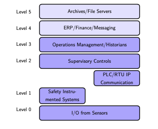
使用chain画瀑布型图
定义如下:
% The Purdue Enterprise Reference Architecture (PERA) model.
% Author: Erno Pentzin (2013)
\documentclass{article}
\usepackage{tikz}
\usetikzlibrary{chains}
\begin{document}

\begin{tikzpicture}[
        scale=0.75,
        start chain=1 going below,
        start chain=2 going right,
        node distance=1mm,
        desc/.style={
                scale=0.75,
                on chain=2,
                rectangle,
                rounded corners,
                draw=black,
                very thick,
                text centered,
                text width=8cm,
                minimum height=12mm,
                fill=blue!30
                },
        it/.style={
                fill=blue!10
        },
        level/.style={
                scale=0.75,
                on chain=1,
                minimum height=12mm,
                text width=2cm,
                text centered
        },
        every node/.style={font=\sffamily}
]

% Levels
\node [level] (Level 5) {Level 5};
\node [level] (Level 4) {Level 4};
\node [level] (Level 3) {Level 3};
\node [level] (Level 2) {Level 2};
\node [level] (Level 1.5) { };
\node [level] (Level 1) {Level 1};
\node [level] (Level 0) {Level 0};

% Descriptions
\chainin (Level 5); % Start right of Level 5
% IT levels
\node [desc, it] (Archives) {Archives/File Servers};
\node [desc, it, continue chain=going below] (ERP) {ERP/Finance/Messaging};
% ICS levels
\node [desc] (Operations) {Operations Management/Historians};
\node [desc] (Supervisory) {Supervisory Controls};
\node [desc, text width=3.5cm, xshift=2.25cm] (PLC) {PLC/RTU IP Communication};
\node [desc, text width=3.5cm, xshift=-4.5cm] (SIS) {Safety Instrumented Systems};
\node [desc, xshift=2.25cm] (IO) {I/O from Sensors};

\end{tikzpicture}

\end{document}
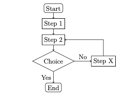
用坐标和position画图
% Author: Laurent Dutriaux
\documentclass[a4paper,11pt]{article}
\usepackage[utf8]{inputenc}
\usepackage{fourier} % Utilisation des polices texte
\usepackage{tikz}
\usetikzlibrary[positioning]
\usetikzlibrary{patterns}
\usepackage[french]{babel} % styles français
\title{A simple Timetable}
\author{Laurent Dutriaux}
\date{\today}
\newcommand{\daywidth}{2.2 cm}
\begin{document}

\maketitle

\begin{tikzpicture}[x=\daywidth, y=-1cm, node distance=0 cm,outer sep = 0pt]
% Style for Days
\tikzstyle{day}=[draw, rectangle,  minimum height=1cm, minimum width=\daywidth, fill=yellow!20,anchor=south west]
% Style for hours
\tikzstyle{hour}=[draw, rectangle, minimum height=1 cm, minimum width=1.5 cm, fill=yellow!30,anchor=north east]

% Styles for events
% Duration of sequences
\tikzstyle{hours}=[rectangle,draw, minimum width=\daywidth, anchor=north west,text centered,text width=5 em]
\tikzstyle{1hour}=[hours,minimum height=1cm]
\tikzstyle{2hours}=[hours,minimum height=2cm]
\tikzstyle{3hours}=[hours,minimum height=3cm]
%Style for type of sequence
\tikzstyle{Ang2h}=[2hours,fill=green!20]
\tikzstyle{Phys2h}=[2hours,fill=red!20]
\tikzstyle{Math2h}=[2hours,fill=blue!20]
\tikzstyle{TIPE2h}=[2hours,fill=blue!10]
\tikzstyle{TP2h}=[2hours, pattern=north east lines, pattern color=magenta]
\tikzstyle{G3h}=[3hours, pattern=north west lines, pattern color=magenta!60!white]
\tikzstyle{Planche}=[1hour,fill=white]
% Positioning labels for days and hours
\node[day] (lundi) at (1,8) {Lundi};
\node[day] (mardi) [right = of lundi] {Mardi};
\node[day] (mercredi) [right = of mardi] {Mercredi};
\node[day] (jeudi) [right = of mercredi] {Jeudi};
\node[day] (vendredi) [right = of jeudi] {Vendredi};
\node[hour] (8-9) at (1,8) {8-9};
\node[hour] (9-10) [below = of 8-9] {9-10};
\node[hour] (10-11) [below= of 9-10] {10-11};
\node[hour] (11-12) [below = of 10-11] {11-12};
\node[hour] (12-13) [below  = of 11-12] {12-13};
\node[hour] (13-14) [below = of 12-13] {13-14};
\node[hour] (14-15) [below = of 13-14] {14-15};
\node[hour] (15-16) [below = of 14-15] {15-16};
\node[hour] (16-17) [below = of 15-16] {16-17};
\node[hour] (17-18) [below = of 16-17] {17-18};
\node[hour] (18-19) [below = of 17-18] {18-19};
%Position of sequences
\node[Ang2h] at (1,10) {Anglais};
\node[Phys2h] at (1,8) {Physique};
\node[Phys2h] at (2,8) {Physique};
\node[Phys2h] at (4,8) {Physique};
\node[Phys2h] at (5,10) {Physique};
\node[Math2h] at (2,10) {Maths};
\node[Math2h] at (2,14) {Maths};
\node[Math2h] at (3,8) {Maths};
\node[Math2h] at (4,10) {Maths};
\node[Math2h] at (5,8) {Maths};
\node[TIPE2h] at (1,14) {TIPE};
\node[TIPE2h] at (1,16) {TIPE};
\node[TIPE2h] at (2,16) {TIPE};
\node[TIPE2h] at (3,10) {TIPE};
\node[TIPE2h] at (5,14) {TIPE};
\node[TIPE2h] at (5,16) {TIPE};
\node[TP2h] at (3,14) {Phys ou SI};
\node[TP2h] at (3,16) {SI ou Phys};
\node[Planche] at (1,13) {Planche};
\node[Planche] at (1,18) {Colle};
\node[Planche] at (4,13.5) {Planche};
\end{tikzpicture}


\end{document}
结果如下: